The source for this post is available here
Intro & Motivation
Yes, there is a mantra, that causality can not be inferred from correlation. No doubt if A correlates with B, it is generally impossible to say if A or B is the cause. Moreover there can be yet another latent variable that cause changes in both. In certains cases however, the directionality determined based on the mechanism. Say, if A is a mutation, B is mRNA abundance, then only A can cause changes in B, but not vice versa. Having said that, let’s consider general cases only when we have no mechanistic knowledge.
Though if there are only two variable, inference of causality without any knowledge about thr mechanism is impossible, the situation becomes more interesting with more variables involved. With more variables, there multiple options which nodes are causal, which are intermediate and which are reactive. Those choices may be non-equivalent with respect to degrees of freedom or in other words - number of input nodes. Given the Occam’s razor the preference should be given to the model with the least input nodes that as effectively exprain the observed variance as models with more input nodes. This is just the intuition. The actual inference relies on formalism like cross-validation and information criteria. Do those approaches guarantee that the inferred causal structure is correct? Absolutely not. However, the result will be the best guess given the data.
Toy Example.
Tree structure.
Simple causal structure in which all the changes originate with the root node A. Only one input node. Yes, the variance can be explained in reverse flow of causality where input nodes are D,E,F and G, however, that will cost extra 3 dergrees of freedom. So, in theory, the algoritm should prefer the structure with only one causal node.
library(bnlearn)
eg <- empty.graph(LETTERS[1:7])
modelstring(eg) <- "[G|C][F|C][E|B][D|B][C|A][B|A][A]"
graphviz.plot(eg)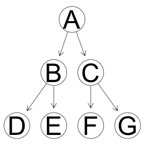
Synthetic data
library(tidyverse)
set.seed(0)
N <- 100 # number of observations per node
sd_ini <- 1 # parameter controlling true effect
sd_sys <- 1 # noise in the system
sd_meas <- 1 # measurement noise
x <- N %>%
   map_df(~tibble(A=rnorm(.,mean=0,sd=sd_ini))) %>%
   # propagating the changes through the nodes
   mutate(B = rnorm(n(), A, sd=sd_sys)) %>%
   mutate(C = rnorm(n(), A, sd=sd_sys)) %>%
   mutate(D = rnorm(n(), B, sd=sd_sys)) %>%
   mutate(E = rnorm(n(), B, sd=sd_sys)) %>%
   mutate(F = rnorm(n(), C, sd=sd_sys)) %>%
   mutate(G = rnorm(n(), C, sd=sd_sys)) %>%
   # adding measurement noise
   mutate_all(funs(rnorm(n(), mean = ., sd = sd_meas)))
Inference
R has a number of packages that deal with causal inference.
bnlearn, pcalg, deal, catnet, gRbase, gRain, rbmn
We’ll give a test to a couple of tools.
bnlearn package
The bnlearn R package has a wonderful collection of algorithms and utilities for causal inference. Speficically the built-in boot.strength function allows to estimate the uncertainities of the inferred edges and their directionality. In the examples below I do not take advantage of uncertainity quantification. However, generally it is a useful guidance if you not sure how believable/reliable the infernce results.
Markov Blanket, iamb implementation
library(parallel)
cl <- makeCluster(detectCores()-1)
clusterSetRNGStream(cl, iseed = 0)
res <- boot.strength(x, cluster = cl, R = 1000, algorithm='iamb')
graphviz.plot(averaged.network(res, threshold = attr(res, "threshold")))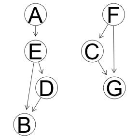
Grow-Shrink Algoritm
res <- boot.strength(x, cluster = cl, R = 1000, algorithm='gs')
graphviz.plot(averaged.network(res))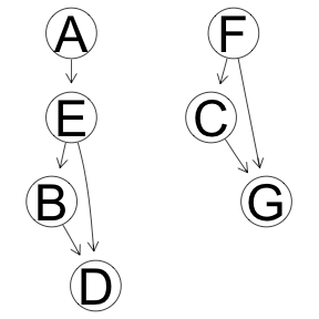
Hill Climbing Optimization
res <- boot.strength(x, cluster = cl, R = 1000, algorithm='hc')
graphviz.plot(averaged.network(res))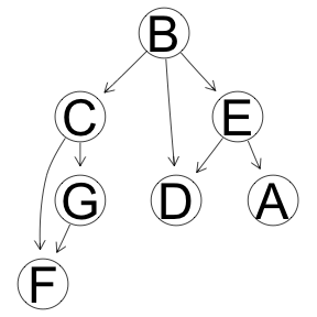
Hill Climbing Optimization. V2
Exactly the same settings as was used for inference of protein signalling network. Causal Protein-Signaling Networks Derived from Multiparameter Single-Cell Data
dx <- discretize(x, method="hartemink", breaks=3, ibreaks=60, idisc="quantile")
res <- boot.strength(dx, cluster = cl, R = 1000, algorithm='hc',
                     algorithm.args = list(score='bde', maximize=10))
graphviz.plot(averaged.network(res))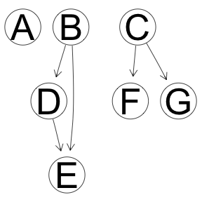
Tabu Optimization
res <- boot.strength(x, cluster = cl, R = 1000, algorithm='tabu')
graphviz.plot(averaged.network(res))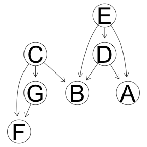
Hybrid Algorithm, ARACNE followed by tabu optimization
res <- boot.strength(x, cluster = cl, R = 1000, algorithm='rsmax2',
                     algorithm.args = list(restrict='aracne',
                                           maximize='tabu'))
graphviz.plot(averaged.network(res))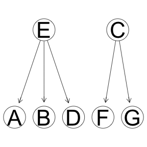
Closing the cluster
stopCluster(cl)pcalg package
library(pcalg)
pc.fit <- pc(suffStat = list(C = cor(x), n = nrow(x)),
             indepTest = gaussCItest,
             skel.method = "stable.fast",
             u2pd = "retry",
             alpha=0.01, labels = colnames(x),
             verbose = FALSE, numCores = detectCores()-1)
graphviz.plot(as.bn(pc.fit))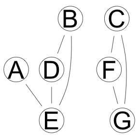
Summary
As evident from the results above, learning the directed acyclic graph structure is not an easy and trivial task. For me it has been mostly been a hit-and-miss process. In the tests above it does not appear that there is clear winner as for the algorithm. Though simulating data with different parameters does result in successful recapitulation of the data structure. For example setting measurement noise to much lower value, 1/10 of the effect, which perhaps unrealistic for biological data, results in proper tree inference using optimizaton-based methods (hc and tabu). I’d note, however, that the main point of this document (at least at this time) is not to provide a guidance as for which approach is the best, but rather provide an example of how to use and evaluate the structure learning tools in R.