The source code of this post is right here.
T-test is one of the basic tests used in biology (and perhaps most others scientific disciplines). However, it is not always interpreted correctly. Hopefully, this small demo will help understanding what the t-test is and what question is answers.
Let’s generate a sample.
set.seed(0)
N <- 5
sample_x <- rnorm(N, mean=0, sd=1)
plot(sample_x, ylim=c(min(0,sample_x),max(0,sample_x)))
abline(h=0, col='red')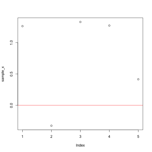
mean(sample_x)## [1] 0.7907182Now the question is if the mean of the sample is different from some value. Typically the question is (or can be reduce down to) if the sample mean is different from zero. A quantity or statistic how far away the sample mean from the NULL mean is so-called t-statistic. \[ t = \frac{\bar{x}-\mu}{\frac{s}{\sqrt{N}}} \]
Let’s compute the t-statitic assuming the NULL mean value = 0.
mu_null <- 0
sample_t_stat <- (mean(sample_x)-mu_null)/(sd(sample_x)/sqrt(N))
print(sample_t_stat)
## [1] 2.420309Hence, our doubt that the mean of the sample is actually not any different from the NULL value can be posed in a more quantitative way. That is:
What is the probability of achieving as big or more extreme t-statistic for a sample with the mean equal to the NULL mean?
Let’s calculate this probability directly by generating a large number of random samples with mean equal to zero.
As a first step we’ll generate random samples with mean equal to the NULL mean. The actual value of the standard deviation at this point does not matter. The t-statistic is scaled by the standard deviation anyway.
N_simulations <- 10000 #1000000
sim_x <- replicate(N_simulations, rnorm(N,mu_null,sd=1))
print(sim_x[,1:5])
## [,1] [,2] [,3] [,4] [,5]
## [1,] -1.539950042 0.7635935 -0.4115108 -0.22426789 0.50360797
## [2,] -0.928567035 -0.7990092 0.2522234 0.37739565 1.08576936
## [3,] -0.294720447 -1.1476570 -0.8919211 0.13333636 -0.69095384
## [4,] -0.005767173 -0.2894616 0.4356833 0.80418951 -1.28459935
## [5,] 2.404653389 -0.2992151 -1.2375384 -0.05710677 0.04672617Calculating t-statistics for the generated random samples.
sim_x_mean_diff <- colMeans(sim_x) - mu_null
sim_x_std_err <- apply(sim_x, 2, sd)/sqrt(N)
sim_t_stats <- sim_x_mean_diff/sim_x_std_err
How often the t-statistic from the random samples is more extreme then the t-statistic of the tested sample?
First let’s make it clear why we are concerned with both higher and lower deviations. It is because we do not say specifically if the sample mean is higher then or lower then the NULL mean. Our sceptical statement is just that it is different. Difference can go both ways - higher and lower. Thus we count deviations on both tails.
hist(sim_t_stats, 100)
abline(v=c(-sample_t_stat,+sample_t_stat), col='red')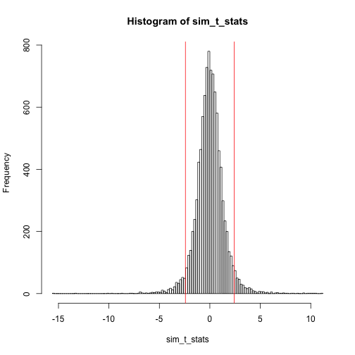
equal_or_more_extreme <- abs(sim_t_stats) >= abs(sample_t_stat)
calc_p_val <- sum(equal_or_more_extreme)/N_simulations
print(calc_p_val)
## [1] 0.0694The actual t-test p-value is:
print(t.test(sample_x)$p.value)## [1] 0.07273875The directly calculated probability of achieving the same or more extreme t-statistic and the p-value from the R’s t.test are quite close!