Intro
Bistability switch that is described here is a chemical reaction system that can jump from one steady state solution into another, drastically different, over a slight change of the input reactant concentration. Presumably a lot of signal transduction pathways downstream of the hormone receptor work as bistability switches. The discussion of bistability switch topic in the context of insulin signaling can be found here and here. The bistability or existence of two drastically difference steady state solutions allows to ignore or filter out relatively small changes of the hormone signals and as soon as it passes a certain threshold turn the system all the way “ON”. A work titled The smallest chemical reaction system with bistability published in BMC Systems Biology (2009) proposes and analyzes the properties of the minimal switch. The model was highlighted as a model of the month at BioModels Database. Here I’ll try to reproduce the model and demonstrate the bistability property.
Underlying abstract chemical reactions
\( S + Y \xrightarrow{k_1} 2 X \)
\( 2 X \xrightarrow{k_2} X + Y \)
\( X + Y \xrightarrow{k_2} Y + P \)
\( Y \xrightarrow{k_3} P \)
ODEs
The set of ordinary differential equations describing the system can be written as follows. The supply of S is constant. The product P does not matter as it is not the reactant (i.e. input for any of the chemical reactions).
\( \frac{dX}{dt} = 2k_{1}SY - k_{2}X^{2} - k_{3}XY - k_{4}X \)
\( \frac{dY}{dt} = -k_{1}SY + k_{2}X^{2} \)
\( \frac{dS}{dt} = 0 \)
Example Simulation
library(deSolve)
library(rootSolve)
library(ggplot2)
library(dplyr)
library(parallel)

minBiStab <- function(Time, State, Pars) {
    with(as.list(c(State, Pars)), {
        dX = 2*k1*S*Y - k2*X^2 - k3*X*Y - k4*X
        dY = -k1*S*Y + k2*X^2
        return(list(c(dX,dY)))
    })
}

pars  <- c(k1 = 8, k2 = 1, k3 = 1, k4 = 1.5, S = 1, P = 1)
yini  <- c(X = 1, Y = 1)
times <- seq(0, 50, by = 1)

res <- ode(yini, times, minBiStab, pars, method = "lsoda")
plot(res)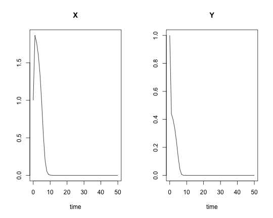
Two distinct steady state solutions
Now we scan the input concentration of S and look for possible steady state solutions. To comprehensively cover possible steady states we will vary the starting concentration of X.
# make all combinations of initial X and S.
xs <- expand.grid(X_ini = 10^seq(0,1,length.out = 100),
                  S = seq(0.5,1.5,length.out = 200))

# parallelized loop through all the combinations
system.time(
    xs <- within(xs,
                 X <- mcmapply(FUN = function(a1,a2)
                     {
                        yini['X'] <- a1
                        pars['S'] <- a2
                        runsteady(yini, time=c(0,Inf), minBiStab, pars)$y['X']
                     }, X_ini, S, mc.cores = 8)))
## user system elapsed
## 296.981 1.848 54.586# plot the results
select(xs,X,S) %>%
# just 4 significant digits to filter out simulation noise
mutate(X = signif(X,4)) %>%
distinct() %>%
ggplot +
aes(x=S, y=X) +
geom_point() +
geom_vline(xintercept = 1.0575, color='red') +
theme_bw()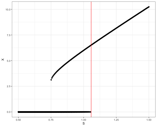
The dots on the plot align into two lines corresponding to the steady state solutions. Note the overlap in the middle. This this the region where two stable solutions are possible. And depends on the initial state of the system, which equilibrium it will evolve to. In case of low concentration of S the system always relaxes to the “lower” steady state solution. As soons as S is above ~1.057 the system becomes unstable and evolve into the “upper” steady state with much higher concentration of X.
Demo
A slight increase of S over the limit point bifurcation results in drastic change of final steady state concentration of X. Reproducing the Figure 3 from the BioModels page.
pars['S'] <- 1.057
res1 <- ode(yini, times, minBiStab, pars, method = "lsoda") %>% as.data.frame
res1$S_ini <- as.character(pars['S'])
pars['S'] <- 1.058
res2 <- ode(yini, times, minBiStab, pars, method = "lsoda") %>% as.data.frame
res2$S_ini <- as.character(pars['S'])
res <- rbind(res1, res2)

ggplot(res, aes(x=time, y=X, color=S_ini)) +
    geom_line(size = 3, alpha = 0.5) +
    theme_bw()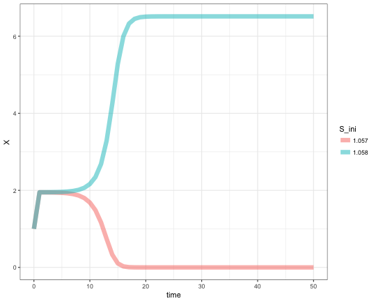
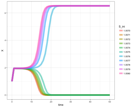
Same type of demonstration, but with a finer stepping. The abuse of %>% pipe is intended. I just enjoy how much cleaner code it makes.
seq(1.057,1.058,length.out = 11) %>%
    mclapply(function(S_ini){
        pars['S'] <- S_ini
        res <- ode(yini, times, minBiStab, pars, method = "lsoda") %>%
            as.data.frame %>%
            mutate(S_ini = sprintf("%.4f",S_ini))},
        mc.cores = 8) %>%
    Reduce(rbind,.) %>%
    ggplot +
        aes(x=time, y=X, color=S_ini) +
        geom_line(size = 3, alpha = 0.5) +
        theme_bw()