Intro
Linear dynamic systems can describe a number of phenomena including system of first-order chemical reactions. An equation describing such systems is as follows:
\( \frac{d\mathbf{x}}{dt} = \mathbf{A}\mathbf{x} \)
Where \(\mathbf{x}\) is the vector of reactant concentrations, \(\mathbf{A}\) is the coefficient matrix corresponding to chemical rate constants.
Simple Case: X1 -> X2 -> X3
Encoding The Reactions As a Graph With igraph
For the sake of simplicity we’ll set all the chemical reaction rate constants to 1. The ODEs corresponding to this simple chain of chemical reactions are:
\( \frac{dX1}{dt} = 1 \cdot X1 + 0 \cdot X2 + 0 \cdot X3 \)
\( \frac{dX2}{dt} = 1 \cdot X1 - 1 \cdot X2 + 0 \cdot X3 \)
\( \frac{dX3}{dt} = 0 \cdot X1 + 1 \cdot X2 + 0 \cdot X3 \)
Firts, let’s encode the reaction graph.
library(igraph)
g <- graph_from_literal( X1 -+ X2 -+ X3 )
E(g)$weight <- rep(1, ecount(g)) # all kinetic contants are 1
plot(g, layout=cbind(c(0,1,2),c(0,0,0)), margin=c(0,0,-2,0))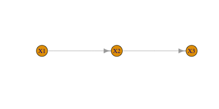
Simulation With deSolve
Extracting matrix with ODE coefficients from the weighted directed graph.
am <- as_adjacency_matrix(g, attr='weight', sparse = FALSE) # influxes
A <- t(am)
diag(A) <- -graph.strength(g, mode = "out") # outfluxes
knitr::kable(A)| X1 | X2 | X3 | |
|---|---|---|---|
| X1 | -1 | 0 | 0 |
| X2 | 1 | -1 | 0 |
| X3 | 0 | 1 | 0 |
The core of the simulation.
library(deSolve)
N <- vcount(g)
yini <- c(1,rep(0,vcount(g)-1)) # first is 1 the rest are 0
names(yini) <- names(V(g))
times <- seq(0, 10, by = 0.01)
deriv_steps <- function(Time, State, Pars){
    list(drop(Pars %*% State))
}
out <- lsoda(yini, times, deriv_steps, A)
Plotting Simulation Results
library(ggplot2)
library(dplyr)
library(tidyr)
as.data.frame(out) %>%
    gather(specie,value,-time) %>%
    ggplot() +
        aes(x=time, y=value, color=specie) +
        geom_line()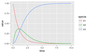
More Complicated Example
Generating Random Reaction Graph
N <- 10 # number of reactants
# Seed controlling random graph
set.seed(2016) # 1, 2000, 2016.
g <- erdos.renyi.game(N, 0.2, directed = TRUE)
V(g)$label <- paste('X', as_ids(V(g)), sep='')
Now we randomize the kinetic rate constants. Note we set them to follow the log-normal distribution. That is all of them will be positive. In the coefficient matrix, the edge weights correspond to kinetic constants of the edges point to a given node. Therefore they will reflect the influx and thus can be only positive. For negative kinetic constant we’ll have to invert the directionality of the edge.
# Seed controlling random number generation for kinetic constants.
set.seed(34660) # 5, 1, 34660.
E(g)$weight <- rlnorm(ecount(g))
Initial concentrations of reactants can be distributed across the species anyway we want. Here we’ll place all the initial concentration into the node with the mose outflux. The code below defines which one is the “source” node for plotting purposes.
V(g)$source <- rep(FALSE,vcount(g))
V(g)$source[which.max(graph.strength(g, mode = "out"))] <- TRUE
Plotting reaction graph with edge weights reflecting the fluxes.
edges_to_curve <- apply(as_edgelist(g), 1, paste, collapse ='_') %in%
    apply(as_edgelist(g)[,c(2,1)], 1, paste, collapse ='_')
set.seed(0) # controlling layout
plot(g,
     vertex.label.cex = 0.7,
     # margin = c(-0.1,-0.1,-0.1,-0.1),
     edge.width=E(g)$weight, edge.curved = edges_to_curve,
     vertex.color=c('gold','orange')[as.numeric(V(g)$source) + 1])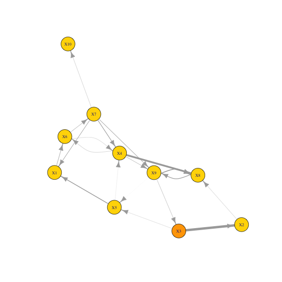
Alternative plotting with ggraph
library(ggraph)
set.seed(5)
ggraph(g, 'igraph', algorithm = 'fr') +
    geom_edge_fan(aes(width=weight, alpha=..index..)) +
    scale_edge_alpha('flows into', guide = 'edge_direction') +
    geom_node_point(size=10, aes(color=source)) +
    geom_node_text(aes(label=label), color=scales::muted('green'), size=4.5) +
    ggforce::theme_no_axes(base.theme = theme_minimal())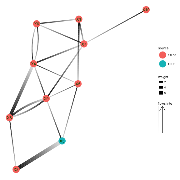
Simulation
Extracting the coefficient matrix.
am <- as_adjacency_matrix(g, attr='weight', sparse = FALSE)
A <- t(am)
diag(A) <- -graph.strength(g, mode = "out")
colnames(A) <- rownames(A) <- V(g)$label
knitr::kable(round(A,2))| X1 | X2 | X3 | X4 | X5 | X6 | X7 | X8 | X9 | X10 | |
|---|---|---|---|---|---|---|---|---|---|---|
| X1 | -1.06 | 0.00 | 0.00 | 0.00 | 1.95 | 0.00 | 1.15 | 0.00 | 0.00 | 0 |
| X2 | 0.00 | -0.46 | 6.46 | 0.00 | 0.00 | 0.00 | 0.00 | 0.00 | 0.00 | 0 |
| X3 | 0.00 | 0.00 | -6.87 | 0.00 | 0.00 | 0.00 | 0.00 | 0.00 | 0.68 | 0 |
| X4 | 0.00 | 0.00 | 0.00 | -6.14 | 0.22 | 0.45 | 1.50 | 0.00 | 0.00 | 0 |
| X5 | 0.00 | 0.00 | 0.41 | 0.00 | -2.17 | 0.00 | 0.00 | 0.00 | 0.04 | 0 |
| X6 | 1.06 | 0.00 | 0.00 | 0.54 | 0.00 | -1.28 | 0.00 | 0.00 | 0.00 | 0 |
| X7 | 0.00 | 0.00 | 0.00 | 0.00 | 0.00 | 0.83 | -4.33 | 0.00 | 0.00 | 0 |
| X8 | 0.00 | 0.46 | 0.00 | 4.82 | 0.00 | 0.00 | 0.00 | -1.63 | 2.24 | 0 |
| X9 | 0.00 | 0.00 | 0.00 | 0.78 | 0.00 | 0.00 | 1.14 | 1.63 | -2.96 | 0 |
| X10 | 0.00 | 0.00 | 0.00 | 0.00 | 0.00 | 0.00 | 0.55 | 0.00 | 0.00 | 0 |
Setting up initial concentrations, defining time interval and finally simulation.
yini <- rep(0,vcount(g))
names(yini) <- V(g)$label
yini[V(g)$source] <- 1
times <- seq(0, 10, by = 0.1)
out <- lsoda(yini, times, deriv_steps, A)
Plotting The Simulation Results
Visualizing the results of the simulation.
as.data.frame(out) %>%
    gather(specie,value,-time) %>%
    mutate(specie = ordered(specie, levels=V(g)$label)) %>%
    ggplot() +
        aes(x=time, y=value, color=specie) +
        geom_line(size=1)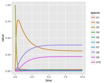
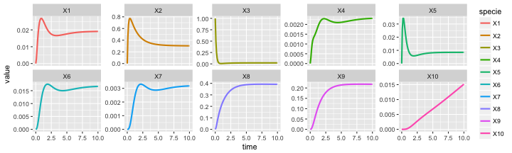
Visualizing trajectory of each specie individually.
as.data.frame(out) %>%
    gather(specie,value,-time) %>%
    mutate(specie = ordered(specie, levels=V(g)$label)) %>%
    ggplot() +
        aes(x=time, y=value, color=specie) +
        geom_line(size=1)  +
        facet_wrap(~ specie, scale = 'free_y', ncol = 5)