The source for this post is available here

Intro & Motivation

A typical way of handling ODEs and systems of ODEs these days is using numerical integration approaches. However, in some cases it is benefitial to have analytical solution. If the system is too complex and non-linear then the feasibility and changes are dwindling. Below I walk through a simple example of system of two linear ODEs. Going through this example helps me to refresh my skills in handling of ODEs, which are getting rusty after being at storage for 25 or so years.

The example is based on the textbook “Mathematical Models in Biology” by Leah Edelstein-Keshet page 140. The books seems to be used by a number of universities as the textbook for the corresponding course. The solution for the example itself is not covered with sufficient details. It took some effort to trace why one equation or statement follows from another. In a meanwhile I found this video from MIT course on Linear Systems rather helpful to connect some dots.

First we’ll solve the initial value problem (aka simulation) using R utilities for numerical integration. Then we’ll walk through derivation of the analytical solution. The analytical solution allows directly calculate the state of the system for each timepoint. After all it is quite satisfying to see that numerical and analytical solutions result in the same answer.

Model Specification

\[ \frac{dx_1}{dt} = x_1 - x_2 \]

\[ \frac{dx_2}{dt} = x_1 + x_2 \]

Let’s set the initial conditions to \(x_1 = 1\) and \(x_2 = 1\).

Numerical Solution

Simulating the system from 0 to 10 seconds with 0.01 second step. Results will be shown later together with analytical solution.

library(deSolve)

# time derivatives of x vector
deriv <- function(Time, State, Pars) {
    with(as.list(c(State, Pars)), {
        dx1 <- x1 - x2
        dx2 <- x1 + x2
        return(list(c(dx1,dx2)))
    })
}

# initial conditions
v_ini  <- c(x1 = 1, x2 = 1)

# time interval to compute the solutions
times <- seq(0, 10, by = 0.01)

# launching solver
out.num <- ode(v_ini, times, deriv, parms = NULL, method = "lsoda")

Analytical Solution

\[\frac{d\vec{x}}{dt} = \left( \begin{array}{r} 1 & -1 \\ 1 & 1 \end{array} \right) \times \vec{x}\]

Eigenvalues

\[\det \left( \begin{array}{r} 1 - \lambda & -1 \\ 1 & 1 - \lambda \end{array} \right) = 0\] \[(1 - \lambda)^2 + 1 = 0\] \[\lambda^2 - 2 \lambda + 2 = 0\]

Accodring to formula for finding roots of quadratic equation:

\[\lambda_{1,2} = \frac{-b \pm \sqrt{b^2 - 4ac}}{2a}\]

The roots are:

\[\lambda_{1,2} = \frac{-(-2) \pm \sqrt{(-2)^2 - 4 \times 1 \times 2}}{2 \times 1}\] \[\lambda_{1,2} = 1 \pm i\]

Note, that the roots are complex conjugates.

Eigenvectors

Eigenvector for the first root is as follows:

\[\left( \begin{array}{r} 1 - \lambda_1 & -1 \\ 1 & 1 - \lambda_1 \end{array} \right) \times \left( \begin{array}{r} v_{11} \\ v_{12} \\ \end{array} \right) = \left( \begin{array}{r} 0 \\ 0 \\ \end{array} \right)\] \[\begin{cases} (1 - (1 + i)) \times v_{11} - v_{12} = 0 \\ v_{11} + (1 - (1 + i)) \times v_{12} = 0 \end{cases}\] \[\begin{cases} -i \times v_{11} - v_{12} = 0 \\ v_{11} - i \times v_{12} = 0 \end{cases}\]

Note, the equations are not independent. The second one can be derived from the first one by multiplying by \(i\). This is always the case when finding eigenvectors. There is always a family of eigenvectors that differ from each other by a constant. We can arbitrary set \(v_{11} = 1\). Thus \(v_{12} = -i\).

Therefore the solutions can be written in the form

\[\vec{x}(t) = \left( \begin{array}{r} 1 \\ -i \end{array} \right) \times e^{(1 + i) \times t}\]

Given the Euler’s formula

\[e^{it} = \cos t + i \sin t\] \[\vec{x}(t) = \left( \begin{array}{r} 1 \\ -i \end{array} \right) \times e^t \times (\cos t + i \sin t)\] \[\vec{x}(t) = e^t \times \left( \begin{array}{r} \cos t + i \sin t \\ -i \cos t + \sin t \end{array} \right)\] \[\vec{x}(t) = e^t \times \left( \left( \begin{array}{r} \cos t \\ \sin t \end{array} \right) + i \times \left( \begin{array}{r} \sin t \\ -\cos t \end{array} \right) \right)\]

General real-valued solutions can be written as combinations of real and imaginary components. There is no need to look for eigenvectors for the second eigenvalue.

\[\vec{x}(t) = e^t \times \left( C_{1} \times \left( \begin{array}{r} \cos t \\ \sin t \end{array} \right) + C_{2} \times \left( \begin{array}{r} \sin t \\ -\cos t \end{array} \right) \right)\]

Constants \(C_1\) and \(C_2\) defined from the initial conditions.

Inferring constants

Substituting \(t = 0\), \(x_1 = 1\) and \(x_2 = 1\) in the general solution equation above.

\[\left( \begin{array}{r} 1 \\ 1 \end{array} \right) = 1 \times \left( C_{1} \times \left( \begin{array}{r} 1 \\ 0 \end{array} \right) + C_{2} \times \left( \begin{array}{r} 0 \\ -1 \end{array} \right) \right)\]

Transforming into system of linear equations:

\[\begin{cases} 1 = 1 \times C_1 + 0 \times C_2 \\ 1 = 0 \times C_1 - 1 \times C_2 \end{cases}\]

Hence \(C_1 = 1\) and \(C_2 = -1\).

Thus the exact solution is:

\[\vec{x}(t) = \left( \begin{array}{r} x_1 \\ x_2 \end{array} \right) = e^t \times \left( \left( \begin{array}{r} \cos t \\ \sin t \end{array} \right) - \left( \begin{array}{r} \sin t \\ -\cos t \end{array} \right) \right)\]

Computing values for analytical solution

# closed form of x(t) function
xt <- function(t){
    v1 <- c(cos(t),  sin(t))
    v2 <- c(sin(t), -cos(t))
    x <- (v1 - v2)*exp(t)
    return(x)
}

library(dplyr)
f <- function(arg) setNames(as.data.frame(t(xt(arg$time))), c("x1", "x2"))
out.anl <- out.num %>%
    as.data.frame %>%
    rowwise %>%
    do(f(.))

Comparing the results

library(ggplot2)
library(viridis)

out.anl <- cbind(type="analytical", time=times, out.anl)
out.num <- cbind(type="numerical", as.data.frame(out.num))
out <- rbind(out.num, out.anl)

ggplot(data=out, aes(x=x1, y=x2, color=time)) +
    geom_path(size=1) + 
    scale_colour_gradientn(colours=viridis(100)) +
    facet_wrap(~ type) +
    theme_gray(base_size = 18)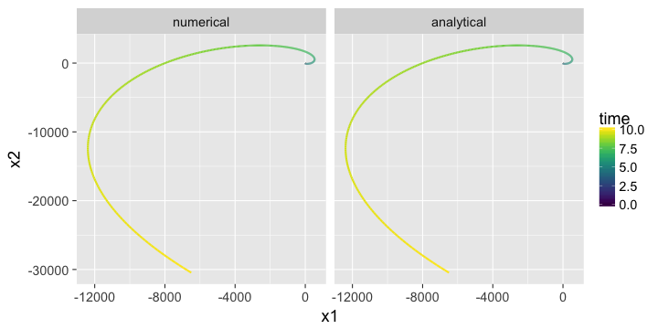

Evidently, they are the same. Math did its magic and numerical integration proved to work well in this case.

Solving it in Mathematica

In[1]:= sol = DSolve[{x1'[t]==x1[t]-x2[t], 
                      x2'[t]==x1[t]+x2[t], 
                      x1[0]==1, 
                      x2[0]==1},
                     {x1[t], x2[t]}, t]

Out[1]= {x1[t]->E^t (Cos[t]-Sin[t]), x2[t]->E^t (Cos[t]+Sin[t])}

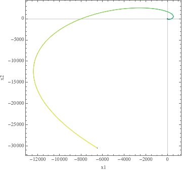
In[2]:= ParametricPlot[{x1[t],x2[t]}/.sol,
                       {t,0,10},
                       PlotRange->All, 
                       AspectRatio->1, 
                       PlotTheme->"Scientific", 
                       FrameLabel->{"x1","x2"},
                       ColorFunctionScaling->True,
                       ColorFunction->Function[{x,y,t},ColorData["BlueGreenYellow"][t]]]

None

Analytical Solution of Linear ODE System with Complex Roots

minimal example from Edelstein-Keshet textbook page 140