The source for this post is available here
Intro & Motivation
When someone needs to perform a linear regression, the first thing that comes to mind is lm function from the the stats R package. However, this linear model relies on assumption that the independent variable x does not contain any measurement error. In case of categorical variables it is probably OK. However, it is still possible that certain points belong to a certain class or factor level with some degree of probability. I won’t consider this case here. Let’s take a look at the situation when x is a continuous variable. If it is a real-world scenario then most likely x is measured with some error. Out of my experience I can point to an example of correlating mRNA vs protein relative abundance. Or correlating protein relative abundance vs some clinical measure. Both values have decent (or at least non-negligible) degree of measurement error. I emphasize both.
Web Resources
A couple of good discussions on that topic can be found here and here.
Simulation
For simulating the example below I picked t-distribution to represent relative protein/mRNA abundances. Typically they don’t just follow normal. Normal component describe mostly measurement noise. Some proteins/mRNA trully change. Thus there is a need for higher then normal probability in the tails. Alternatively one can simulate relative protein abundances with a two-component distribution - combination of normal and uniform.
set.seed(0)
x0 <- rt(2000, 10)
x <- rnorm(length(x0), x0, 1)
y <- rnorm(length(x0), x0, 1)
plot(x,y)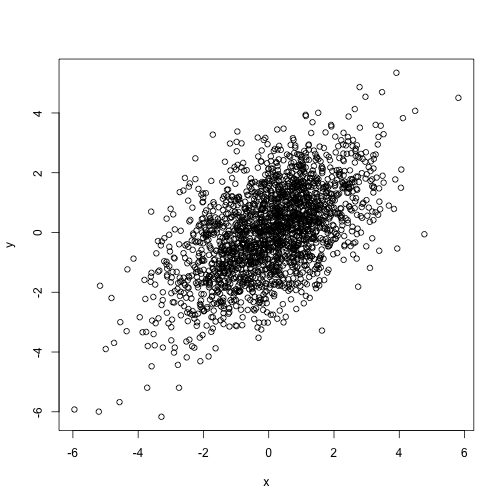
Regular linear model
Regular linear model lm relies on oridinary least squares approach. It assumed that x does not have any error. The goodness of fit calculated as squared difference between observed and fitted y values.
m1 <- lm(y ~ x)
plot(x,y)
abline(m1, col="red")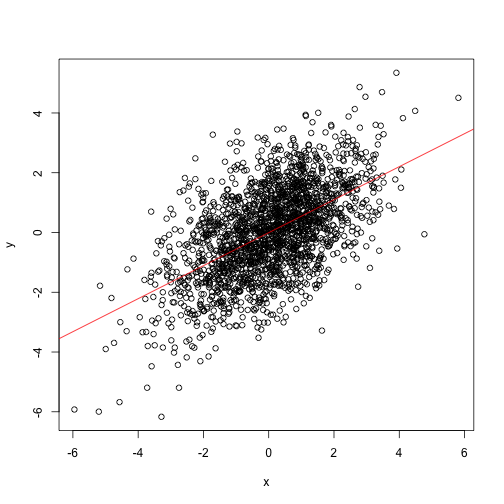
The slope of that line doesn’t look right. Isn’t it?
Total least squares leveraging PCA
It is fairly intuitive that PCA can be one helpful approach here. The most variance is along the x vs y slope. Thus PCA will rotate the scatterplot such that first principal component will be along the slope.
v <- prcomp(cbind(x, y))$rotation
beta <- v[2,1]/v[1,1]

plot(x,y)
abline(m1, col="red")
abline(a = 0, b = beta, col="green")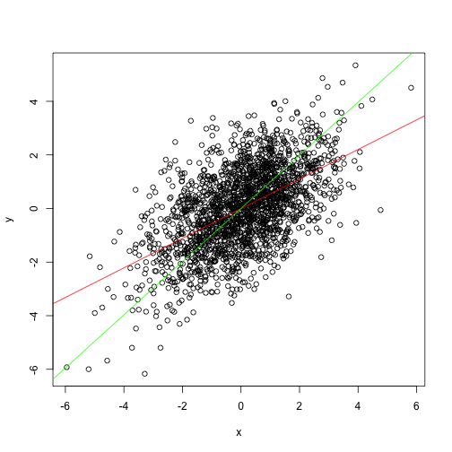
TLS regression pracma::odregress
pracma package has a dedicated function for total least squares or alternatively called orthogonal distance regression.
library(pracma)
m2 <- odregress(x, y)

plot(x,y)
abline(m1, col="red")
abline(a = 0, b = beta, col="green")
abline(b=m2$coeff[1], a=m2$coeff[2], col="cyan")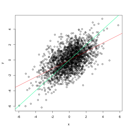
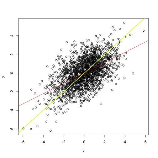
Deming regression
The most general approach for hangling such scenarios would be Deming regression. In its simplest form with default settings it is equivalent to total least squares.
library(MethComp)## Loading required package: nlmem3 <- Deming(x, y)
plot(x,y)
abline(m1, col="red")
abline(a = 0, b = beta, col="green")
abline(b=m2$coeff[1], a=m2$coeff[2], col="cyan")
abline(a=m3["Intercept"], b=m3["Slope"], col="yellow", lwd=2)